前言

在机器学习以及深度学习中，Normalization解决的是Internal Covariate Shift，解决梯度弥散的问题，提高训练速度。
另一方面，在机器学习模型中，如果模型参数太多了，而训练样本又太少了，训练出来的模型容易过拟合。为了避免这种情况的发生，使用Dropout可以有效地缓解过拟合的发生，在一定程度上达到正则化的效果。Dropout可以作为训练神经网络的一种Trick选择。在每个训练批次中，通过忽略一半的特征检测器（让一半的隐层节点值为0），可以明显地减少过拟合现象。这种方式可以减少特征检测器（隐层节点）间的相互作用，检测器相互作用是指某些检测器依赖其他检测器才能发挥作用。

现在我们一起来讨论下训练阶段的前向传播和后向传播以及推理阶段的Normalization和Dropout是如何计算的。

Batch Normalization

Normalization可以参考之前写的一篇文章：深度学习 Normalization。

前向传播

BatchNormalization前向传播比较简单，首先求得mini-batch的均值和方法，然后对$x$进行归一化，最后做尺度转换和变换。整个计算过程如下图所示：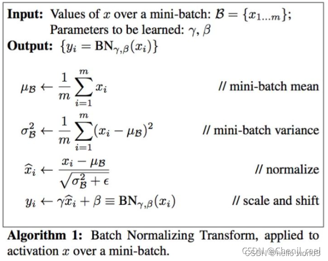

后向传播

BN后向传播的计算可以参考这篇文章：Understanding the backward pass through Batch Normalization Layer和笔记：Batch Normalization及其反向传播。BN的后向传播可以通过以下这张图理解：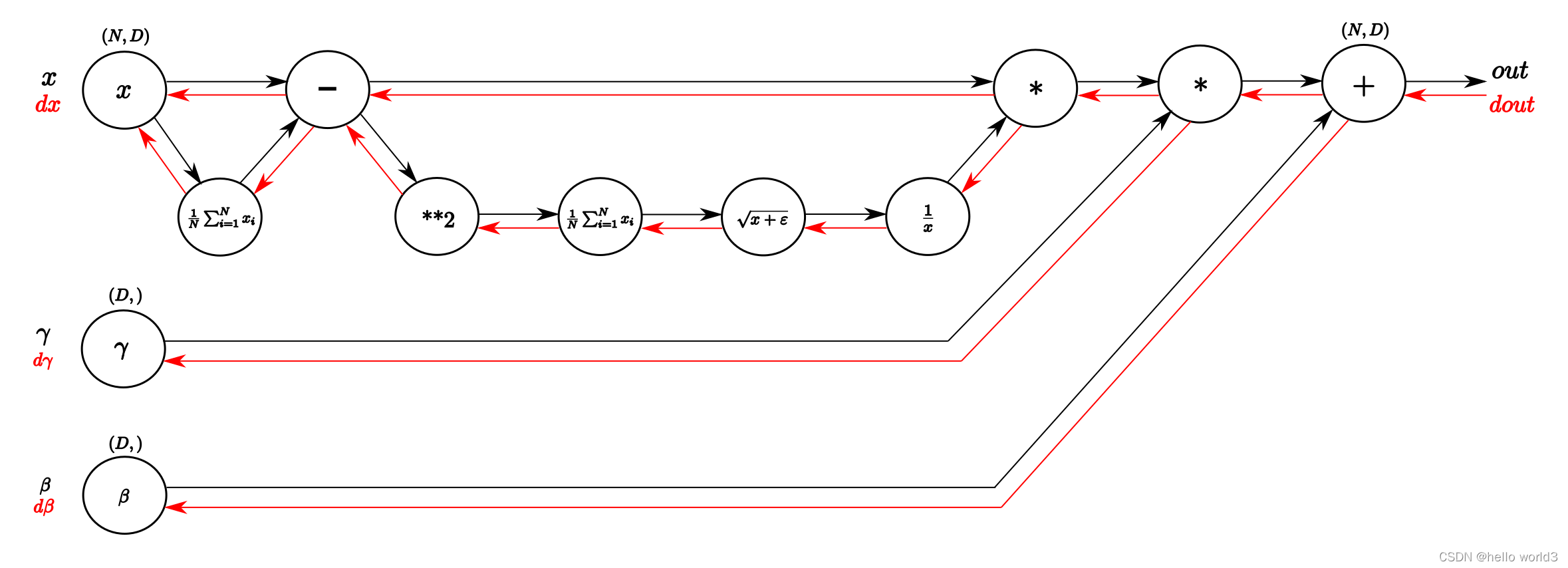

从左向右是前向传播的过程，输入是矩阵$X$、$\gamma$以及$\beta$。反过来从右向左就是它的反向传播过程，沿着红色的箭头进行链式求导。在反向求导的过程中，有一点需要了解的是链式求导，链式求导大致过程如下图所示：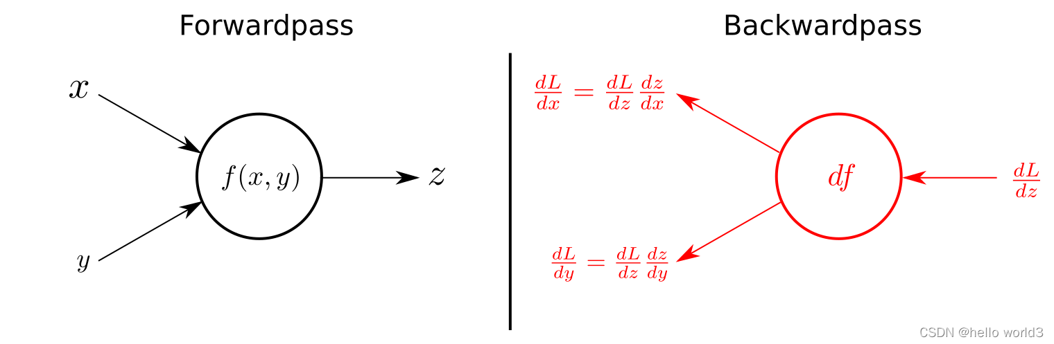

接下来我们一步步看反向传播的过程。
第一步：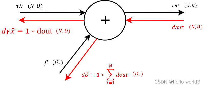

这一步主要对加法进行求导，类似$f=x+y$分别对$x$和$y$进行求导，得到的值为1。接着对所有输出进行求和之后即可得到参数$\beta$的值。

第二步：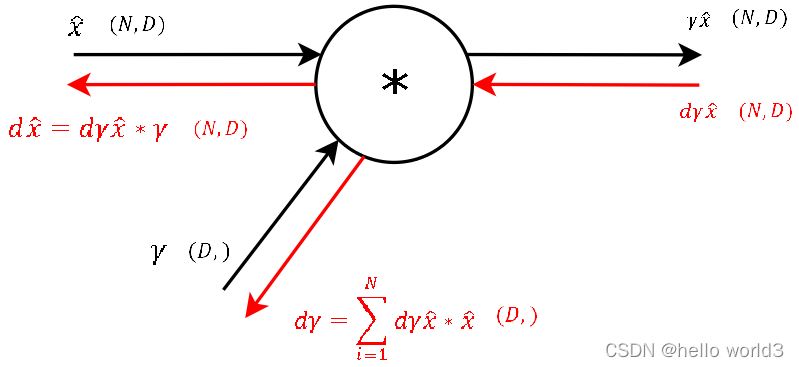

这一步主要类似$f=x\times y$分别对$x$和$y$进行求导，得到的结果是对其中一个输入的导数是另一个输入变量。 对于$\gamma$参数，此时类似$\beta$操作，只需要把梯度求和即可得出。现在求得$\gamma$参数后，剩下只需要对输入$x$的参数进行调整即可。

第三步：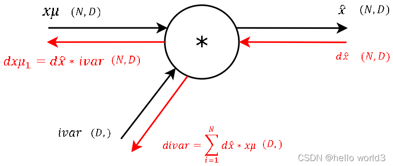

第四步：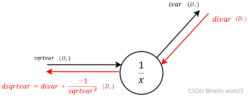

第五步：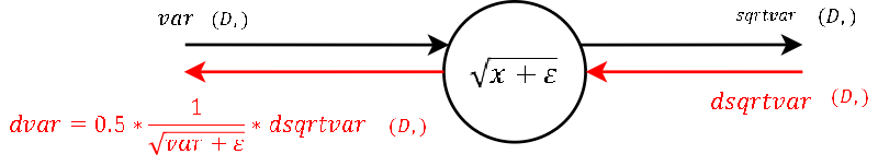

第六步：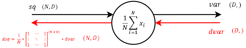

The calculation of the derivative of this steps local gradient might look unclear at the very first glance. But it’s not that hard at the end. Let’s recall that a normal summation gate (see step 9) during the backward pass only transfers the gradient unchanged and evenly to the inputs. With that in mind, it should not be that hard to conclude, that a column-wise summation during the forward pass, during the backward pass means that we evenly distribute the gradient over all rows for each column. And not much more is done here. We create a matrix of ones with the same shape as the input sq of the forward pass, divide it element-wise by the number of rows (thats the local gradient) and multiply it by the gradient from above.

第七步：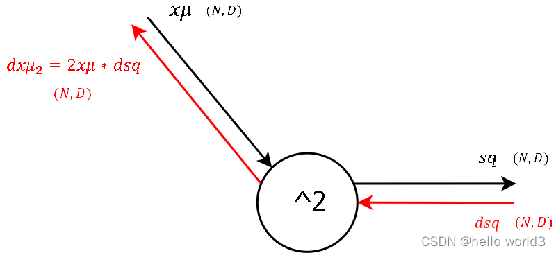

第八步：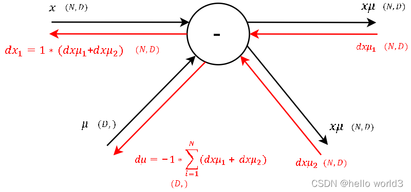

第九步：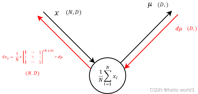

第十步：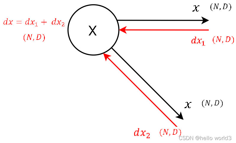

import numpyas npdefbatchnorm_forward(x, gamma, beta, bn_param):# read some useful parameter
    N, D= x.shape
    eps= bn_param.get('eps',1e-5)
    momentum= bn_param.get('momentum',0.9)
    running_mean= bn_param.get('running_mean', np.zeros(D, dtype=x.dtype))
    running_var= bn_param.get('running_var', np.zeros(D, dtype=x.dtype))# BN forward pass
    sample_mean= x.mean(axis=0)
    sample_var= x.var(axis=0)
    x_=(x- sample_mean)/ np.sqrt(sample_var+ eps)
    out= gamma* x_+ beta# update moving average
    running_mean= momentum* running_mean+(1-momentum)* sample_mean
    running_var= momentum* running_var+(1-momentum)* sample_var
    bn_param['running_mean']= running_mean
    bn_param['running_var']= running_var# storage variables for backward pass
    cache=(x_, gamma, x- sample_mean, sample_var+ eps)return out, cachedefbatchnorm_backward(dout, cache):# extract variables
    N, D= dout.shape
    x_, gamma, x_minus_mean, var_plus_eps= cache# calculate gradients
    dgamma= np.sum(x_* dout, axis=0)
    dbeta= np.sum(dout, axis=0)

    dx_= np.matmul(np.ones((N,1)), gamma.reshape((1,-1)))* dout
    dx= N* dx_- np.sum(dx_, axis=0)- x_* np.sum(dx_* x_, axis=0)
    dx*=(1.0/N)/ np.sqrt(var_plus_eps)return dx, dgamma, dbeta

推理阶段

在训练阶段，BN层的$\mu$和${\sigma }^2$都是基于当前batch的训练数据，然而在预测阶段，可能只需要预测一个样本或者很少的样本，此时$\mu$和${\sigma }^2$的计算有一定的偏估计，这时候利用BN训练好模型后，保留了mini-batch训练数据在网络中每一层的${\mu }_{batch}$与${\sigma }_{batch}^2$。此时使用整个样本的统计量来对预测数据进行归一化。除了这种方法，还可以对可以对train阶段每个batch计算的mean/variance采用指数加权平均来得到test阶段mean/variance的估计。

Dropout

Dropout的工作原理是在前向传播的过程中，让某个神经元的激活值以一定的概率$p$停止工作，可以使模型泛化性能更强。

前向传播

1. 首先随机（临时）删除网络中一半的隐藏神经元，输入输出神经元保持不变。
2. 输入$x$通过修改后的网络前向传播，然后将损失结果反向传播，更新未被删除神经元的参数。
3. 恢复被删除的神经元，重复1、2步。

后向传播

后向传播在前向传播的时候已经阐明了。

推理阶段

推理过程则无需考虑，恢复完整的网络结构即可。

扩展

Batch Renormalization

参考论文：Batch Renormalization: Towards Reducing Minibatch Dependence in Batch-Normalized Models

这篇论文主要阐述了Batch Normalization的几个问题：

• 对于mini-batch，batch normalization的效果可能不是特别好
• 推理阶段的均值和方差采用训练阶段每个batch均值和方差的平均值，假设每个batch都不是同分布，这点会产生误差。

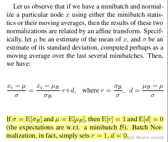
而这篇论文为了保证训练阶段与推理阶段的BN的等效性，解决minibatch的问题，提出Batch Renormalization，具体算法如下：

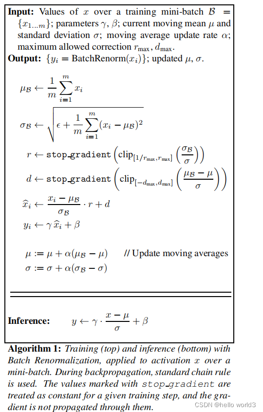
后向传播：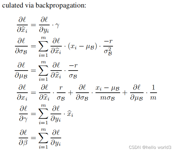

效果：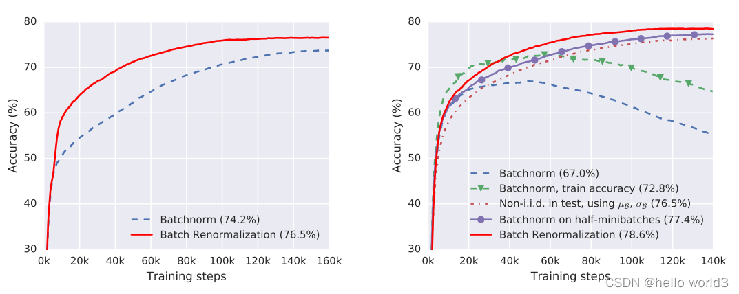

相关代码实现可以参考：https://github.com/titu1994/BatchRenormalization

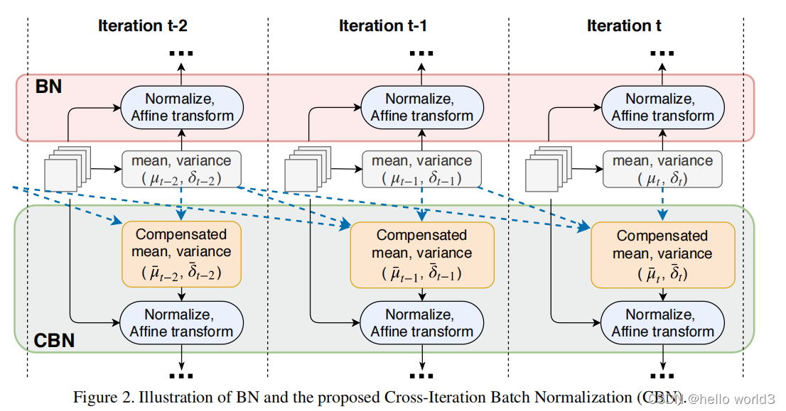
Cross-Iteration Batch Normalization

论文：CBN：Cross-Iteration Batch Normalization。 代码地址：https://github.com/Howal/Cross-iterationBatchNorm。该论文分析了各种Normalization的优缺点，有Batch Normalization，Group Normalization，Instance Normalization的不足，提出了一种Normalization：CrossIteration Batch Normalization (CBN)。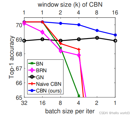

文章也提到上面的Batch Renormalization(BRN)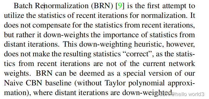

CBN方法与BN比较如下：