手写数字识别,机器学习“分类”学习笔记—来自Geron的《机器学习实战》
图片识别领域的“hello word”
MNIST
获取MNIST代码,70000张手写数字的图片----28x28个像素0-255黑白像素点
Scitkit-Learn 加载数据集通常为字典结构
(这里需要下载数据集,时间比较长,data_home为保存路径,事先设定好路径之后就不会找不到数据存放在那了)
from sklearn.datasets import fetch_openml
mnist = fetch_openml('mnist_784',version=1,data_home='./datasets',as_frame=False)
mnist.keys()
dict_keys(['data', 'target', 'frame', 'categories', 'feature_names', 'target_names', 'DESCR', 'details', 'url'])注意:这里mnist = fetch_openml(‘mnist_784’,version=1,data_home=’./datasets’,as_frame=False )这里书上是没有as_frame=False的,当没有这句话时,后面是读不出来数据的
去查看了git-hub上的代码是这样说的
Warning: since Scikit-Learn 0.24, fetch_openml() returns a Pandas DataFrame by default. To avoid this and keep the same code as in the book, we use as_frame=False.
可见是版本更新之后出现的与数据格式的不同
X,y = mnist["data"],mnist["target"]
X.shape
(70000, 784)y.shape(70000,)使用Matplotlib中的imgshow()将图片显示出来
import matplotlib as mpl
import matplotlib.pyplot as plt
some_digit = X[0]
some_digit_image = some_digit.reshape(28,28)

plt.imshow(some_digit_image,cmap="binary")
plt.axis("off")
plt.show()

y[0]
'5'这里标签是字符,机器学习希望标签为数字
import numpy as np
y = y.astype(np.uint8)
# 划分训练集和测试集
X_train, X_test, y_train, y_test = X[:60000],X[60000:],y[:60000],y[60000:]训练二元分类器
从二分类问题开始,区分数字5与非5
用随机梯度下降分类器SGD,SGD优势在于能够有效处理非常大型的数据集
y_train_5=(y_train == 5)
t_test_5 = (y_test == 5)

from sklearn.linear_model import SGDClassifier
sgd_clf = SGDClassifier(random_state = 27) # 27 是随机数种子,这里自己定义就好
sgd_clf.fit(X_train,y_train_5)SGDClassifier(random_state=27)sgd_clf.predict([some_digit])#这里就是上面图片所示的数字5array([ True])性能测量
使用交叉验证测量准确率
用cross_val_score()函数来评估SGDClassifier模型,采用K折叠验证法(三个折叠)
from sklearn.model_selection import cross_val_score
cross_val_score(sgd_clf,X_train,y_train_5,cv=3,scoring="accuracy")
array([0.9436 , 0.95535, 0.9681 ])折叠交叉的正确率超过93%,看起来很高的样子,但是如果把每一个测试集都语言成非5的话,正确率将达到90%,如下所示
from sklearn.base import BaseEstimator

class Never5Classifier(BaseEstimator):
    def fit(self,X,y=None):
        return self
    def predict(self,X):
        return np.zeros((len(X),1),dtype=bool)#预测全为0

never_5_clf = Never5Classifier()
cross_val_score(never_5_clf,X_train,y_train_5,cv=3,scoring="accuracy")
array([0.91125, 0.90855, 0.90915])这说明用准确率通常无法成为分类器的首要性能指标,所欲需要其他的指标来评判一个预测模型的好坏
混淆矩阵
统计类别A实例被分成为实例B类别的次数
from sklearn.model_selection import cross_val_predict

y_train_pred = cross_val_predict(sgd_clf,X_train,y_train_5,cv=3)

from sklearn.metrics import confusion_matrix
confusion_matrix(y_train_5, y_train_pred)
array([[52775, 1804],
[ 855, 4566]], dtype=int64)上面的结果矩阵就是混淆矩阵,预测非5正确的有52775个(真负类TN),将非5预测为5的有1804个(假正类FP),将5预测为非5的有855个(假负类FN)。正确预测非5的有4566个(真正类TP)。可见预测结果的准确率并不是我们想要的,但是上述的结果的准确率却高达93%,因此,我们不应该用正确率来衡量一个模型的好坏
精度和召回率
精 度 = T P T P + F P 精度=\frac{TP}{TP+FP}精度=TP+FPTP 即正确预测的准确率
召
回
率
=
T
P
T
P
+
F
N
召回率=\frac{TP}{TP+FN}召回率=TP+FNTP 分类器正确检测到正类实例的比率
from sklearn.metrics import precision_score, recall_score
print(precision_score(y_train_5,y_train_pred))
recall_score(y_train_5,y_train_pred)
0.7167974882260597
0.8422800221361373这里精度和准确率代表啥呢?当它说一张图片是5的时候,只有72.9%的概率是准确的,也只有75.6%的数字5被它检测出来了
这时就需要一个评价指标综合精度和准确率对模型进行评价,F1-score就诞生了,F1分数是精度和召回率的谐波平均值。
F
1
=
2
1
精
度
+
1
召
回
率
=
2
×
精
度
×
召
回
率
精
度
+
召
回
率
=
T
P
T
P
+
F
N
+
F
P
2
F_1=\frac{2}{\frac{1}{精度}+\frac{1}{召回率}}=2\times\frac{精度\times召回率}{精度+召回率}=\frac{TP}{TP+\frac{FN+FP}{2}}F1=精度1+召回率12=2×精度+召回率精度×召回率=TP+2FN+FPTP
from sklearn.metrics import f1_score
f1_score(y_train_5,y_train_pred)0.7744890170469002精度/召回率权衡
Scikit-learn不能直接设置F1score的阈值,但是可以访问它用于预测的决策分数。如下所示
y_scores = sgd_clf.decision_function([some_digit])
y_scoresarray([1066.49326077])threshold = 0
y_some_digit_pred = (y_scores > threshold)
y_some_digit_predarray([ True])threshold = 1100
y_some_digit_pred = (y_scores > threshold)
y_some_digit_predarray([False])SGDClassifier分类器使用的阈值,这证明了提高阈值可以降低召回率。
下面来获取训练集中所有实例的分数
y_scores = cross_val_predict(sgd_clf,X_train,y_train_5,cv=3,method="decision_function")
#计算所有可能的阈值的精度和召回率
from sklearn.metrics import precision_recall_curve
precisions,recalls,thresholds = precision_recall_curve(y_train_5,y_scores)

#使用Matplotlib绘制精度和召回度相对于阈值的函数图
def plot_precision_recall_vs_threshold(precision,recalls,thresholds):
    plt.plot(thresholds,precision[:-1],"b--",label="Precision")
    plt.plot(thresholds,recalls[:-1],"g-",label="Recall")
    plt.legend(loc="center right", fontsize=16)
    plt.xlabel("Threshold", fontsize=16)
    plt.grid(True)
    plt.axis([-50000, 50000, 0, 1])

plot_precision_recall_vs_threshold(precisions,recalls,thresholds)
plt.show()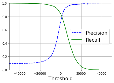
#精度召回率的函数图
def plot_precision_vs_recall(precisions, recalls):
    plt.plot(recalls, precisions, "b-", linewidth=2)
    plt.xlabel("Recall", fontsize=16)
    plt.ylabel("Precision", fontsize=16)
    plt.axis([0, 1, 0, 1])
    plt.grid(True)
recall_90_precision = recalls[np.argmax(precisions >= 0.90)]
plt.figure(figsize=(8, 6))
plot_precision_vs_recall(precisions, recalls)
plt.plot([recall_90_precision, recall_90_precision], [0., 0.9], "r:")
plt.plot([0.0, recall_90_precision], [0.9, 0.9], "r:")
plt.plot([recall_90_precision], [0.9], "ro")
plt.show()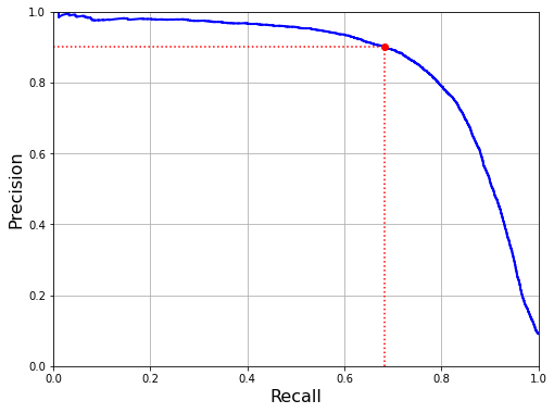
#将精度设置为90%

threshold_90_precision = thresholds[np.argmax(precisions >= 0.90)]
y_train_pred_90 = (y_scores >= threshold_90_precision)
precision_score(y_train_5,y_train_pred_90)0.9001457725947521recall_score(y_train_5,y_train_pred_90)0.6834532374100719所以如果有人对你需求为99%的精度,你就可以反问一句:“召回率是多少?”杀他一个措手不及
ROC曲线
ROC曲线绘制的是真正类率(也是召回率)与假正类率(FPR),FPR是被错误分为正类的负类实例的比率=1-TNR
ROC曲线绘制的是灵敏度(召回率)和(1-特异度)的关系
from sklearn.metrics import roc_curve
fpr,tpr,threshold = roc_curve(y_train_5,y_scores)

def plot_roc_curve(fpr,tpr,label = None):
    plt.plot(fpr,tpr,linewidth=2,label=label)
    plt.plot([0,1],[0,1],'k--')
    plt.axis([0, 1, 0, 1])
    plt.xlabel('False Positive Rate (Fall-Out)', fontsize=16)
    plt.ylabel('True Positive Rate (Recall)', fontsize=16)
    plt.grid(True)

plot_roc_curve(fpr,tpr)
plt.show()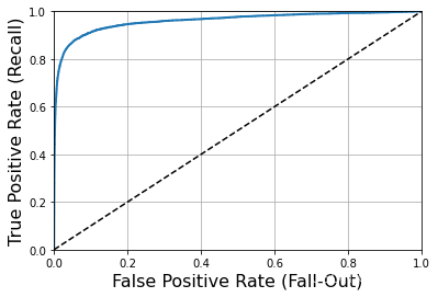
还有一种比较分类器的方法就是测量曲线下面积(AUC),完美的AUC=1,纯随机分类器AUC=0.5
from sklearn.metrics import roc_auc_score
roc_auc_score(y_train_5,y_scores)0.9604387033143528当正类非常少见或者你更关注正类而不是假负类的时候应该选择,PR曲线,反之则为ROC曲线。
随机森林分类器
from sklearn.ensemble import RandomForestClassifier

forest_clf = RandomForestClassifier(random_state=27)
y_probas_forest =cross_val_predict(forest_clf,X_train,y_train_5,cv=3,method="predict_proba")
y_scores_forest = y_probas_forest[:,1]
fpr_forest,tpr_forest,thresholds_forest = roc_curve(y_train_5,y_scores_forest)

plt.plot(fpr,tpr,"b:",label="SGD")
plot_roc_curve(fpr_forest,tpr_forest,"Random forest")
plt.legend(loc="lower right")
plt.show()
[外链图片转存失败,源站可能有防盗链机制,建议将图片保存下来直接上传(img-jkTeibfC-1638890528716)(output_46_0.png)]
roc_auc_score(y_train_5,y_scores_forest)0.9983414796223264RandomForestClassifier的ROC曲线看起来比SGDClassifier好很多,它里左上角更近,因此它的ROC-AUC分数也高很多
多类分类器
多分类器分为OvO与OvR,这里使用了OvO,也就是这里的多分类器实际上是分类了45个二分类器
from sklearn.svm import SVC

svm_clf = SVC()
svm_clf.fit(X_train,y_train)
svm_clf.predict([some_digit])
array([5], dtype=uint8)some_digit_scores = svm_clf.decision_function([some_digit])
some_digit_scoresarray([[ 1.72501977, 2.72809088, 7.2510018 , 8.3076379 , -0.31087254,
9.3132482 , 1.70975103, 2.76765202, 6.23049537, 4.84771048]])最高分确实是5这个类别
np.argmax(some_digit_scores)5当训练分类器的时候,目标类的列表会储存在classes属性中,按照值的大小顺序排列
svm_clf.classes_array([0, 1, 2, 3, 4, 5, 6, 7, 8, 9], dtype=uint8)若想要强制Scikit-learn使用一对一或者一对剩余策略,可以使用OneVsOneClasssifier或者OneVsRestClassifier类。
from sklearn.multiclass import OneVsRestClassifier

ovr_clf = OneVsRestClassifier(SVC())
ovr_clf.fit(X_train,y_train)
ovr_clf.predict([some_digit])
array([5], dtype=uint8)len(ovr_clf.estimators_)10训练SGDClassifier或者RandomForestClassifier的多分类问题与上面情况类似
sgd_clf.fit(X_train,y_train)
sgd_clf.predict([some_digit])
#SGD分类器能够直接将实例分为多个类,所以就不用决定是OvO还是OvR了
array([3], dtype=uint8)sgd_clf.decision_function([some_digit])array([[-16594.39761568, -22903.10175344, -15146.89058029,
1185.04960985, -20053.1928768 , 508.90204236,
-23168.38978204, -19229.31273118, -10995.42427777,
-5902.26098972]])要评估这个分类器的话,与往常一样,使用交叉验证来评估
cross_val_score(sgd_clf,X_train,y_train,cv=3,scoring="accuracy")array([0.8714 , 0.8818 , 0.86235])将输入进行简单缩放,可以进一步提高准确率
from sklearn.preprocessing import StandardScaler
scaler = StandardScaler()
X_train_scaled = scaler.fit_transform(X_train.astype(np.float64))
cross_val_score(sgd_clf,X_train_scaled,y_train,cv=3,scoring="accuracy")
array([0.90025, 0.89075, 0.901 ])误差分析
如果要对模型进行进一步的改进,方法之一就是分析其错误类型,首先看看混淆矩阵
y_train_pred = cross_val_predict(sgd_clf,X_train_scaled,y_train,cv=3)
conf_mx = confusion_matrix(y_train,y_train_pred)
conf_mx
array([[5572, 0, 23, 6, 9, 48, 36, 6, 222, 1],
[ 0, 6399, 39, 21, 4, 44, 4, 7, 214, 10],
[ 27, 27, 5243, 90, 71, 24, 65, 36, 368, 7],
[ 22, 17, 117, 5217, 2, 209, 26, 39, 411, 71],
[ 10, 14, 48, 8, 5190, 12, 35, 24, 338, 163],
[ 26, 15, 29, 167, 54, 4449, 73, 14, 536, 58],
[ 30, 15, 46, 2, 44, 96, 5547, 3, 134, 1],
[ 20, 11, 50, 25, 49, 12, 3, 5692, 192, 211],
[ 16, 65, 51, 89, 3, 126, 24, 10, 5425, 42],
[ 21, 18, 30, 61, 116, 36, 1, 178, 382, 5106]],
dtype=int64)数字很多看起来挺麻烦,使用matplotlib的matshow()来呈现
plt.matshow(conf_mx,cmap=plt.cm.gray)
plt.show()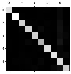
比较错误率
row_sums = conf_mx.sum(axis=1,keepdims = True)
norm_conf_mx = conf_mx / row_sums
用0填充对角线,只保留错误,重新绘制结果
np.fill_diagonal(norm_conf_mx,0)
plt.matshow(norm_conf_mx,cmap=plt.cm.gray)
plt.show()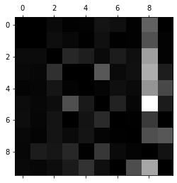
分析混淆矩阵通常可以帮助深入了解如何改进分类器。