历史文章：

1、python底层实现KNN:https://blog.csdn.net/cccccyyyyy12345678/article/details/117911220

2、Python底层实现决策树：https://blog.csdn.net/cccccyyyyy12345678/article/details/118389088

3、Python底层实现贝叶斯：https://blog.csdn.net/cccccyyyyy12345678/article/details/118411638

前言

实现线性回归的方法包括梯度下降法和正规方程，本文只介绍梯度下降法。

本文实现了普通梯度下降多元线性回归和带L2正则化的梯度下降多元线性回归。正则化可以降低高次项的权重系数，从而防止过拟合。

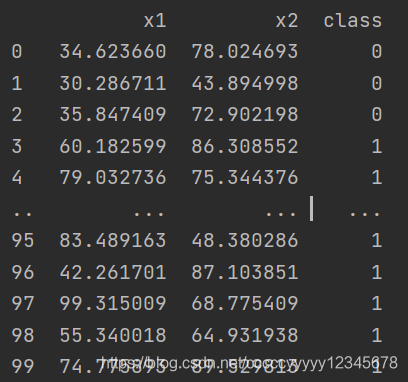
1、导入数据

数据如下：

导入数据使用pandas库，代码如下：

def read_xlsx(path):
    data = pd.read_excel(path)
    print(data)
    return data

2、归一化

归一化方法与KNN中用到的方法相同，这里用归一化消除量纲的目的是使得梯度下降的速度更快。

def MinMaxScaler(data):
    col = data.shape[1]
    for i in range(0, col-1):
        arr = data.iloc[:, i]
        arr = np.array(arr)
        min = np.min(arr)
        max = np.max(arr)
        arr = (arr-min)/(max-min)
        data.iloc[:, i] = arr
    return data

3、划分训练集和测试集

def train_test_split(data, test_size=0.2, random_state=None):
    col = data.shape[1]
    x = data.iloc[:, 0:col-1]
    y = data.iloc[:, -1]
    x = np.array(x)
    y = np.array(y)
    # 设置随机种子，当随机种子非空时，将锁定随机数
    if random_state:
        np.random.seed(random_state)
        # 将样本集的索引值进行随机打乱
        # permutation随机生成0-len(data)随机序列
    shuffle_indexs = np.random.permutation(len(x))
    # 提取位于样本集中20%的那个索引值
    test_size = int(len(x) * test_size)
    # 将随机打乱的20%的索引值赋值给测试索引
    test_indexs = shuffle_indexs[:test_size]
    # 将随机打乱的80%的索引值赋值给训练索引
    train_indexs = shuffle_indexs[test_size:]
    # 根据索引提取训练集和测试集
    x_train = x[train_indexs]
    y_train = y[train_indexs]
    x_test = x[test_indexs]
    y_test = y[test_indexs]
    # 将切分好的数据集返回出去
    # print(y_train)
    return x_train, x_test, y_train, y_test

4、梯度下降线性回归

（1）普通梯度下降

梯度下降法是迭代法的一种，可以用与求解最小二乘问题。直接用最小二乘法计算得到的过程即正规方程。而梯度下降则是一步一步逼近最优解（也可能是局部最优解）。

损失函数用真实值和预测值的均方误差来定义

def costFunction(x, y, theta):
    m = len(x)
    J = np.sum(np.power(np.dot(x, theta) - y, 2)) / (2 * m)
    return J

固定步长和迭代次数进行梯度下降:

def gradeDesc(x,y,alpha=0.01,iter_num=2000):
    x = np.array(x)
    y = np.array(y).reshape(-1, 1)
    m = x.shape[0]
    n = x.shape[1]
    theta = np.zeros(n + 1).reshape(-1, 1)
    c = np.ones(m).transpose() #构建m行1列 x0=1
    x = np.insert(x, 0, values=c, axis=1)
    costs = np.zeros(iter_num)   # 初始化cost, np.zero生成1行iter_num列都是0的矩阵
    for i in range(iter_num):
        for j in range(n):
            theta[j] = theta[j] + np.sum((y - np.dot(x, theta)) * x[:, j].reshape(-1, 1)) * alpha / m
        costs[i] = costFunction(x, y, theta)
    return theta, costs

（2）带L2正则化梯度下降

L2正则化需要最小化权值，因此引入惩罚项来控制权值。

def l2costFunction(x, y, lamda, theta):
    m = len(x)
    J = np.sum(np.power((np.dot(x, theta) - y), 2)) / (2 * m) + lamda * np.sum(np.power(theta, 2))
    return J

梯度下降过程中唯一的不同就是求导后的公式

def l2gradeDesc(x, y, alpha, iter_num, lamda):
    x = np.array(x)
    y = np.array(y).reshape(-1, 1)
    m = x.shape[0]
    n = x.shape[1]
    theta = np.zeros(n + 1).reshape(-1, 1)
    c = np.ones(m).transpose()
    x = np.insert(x, 0, values=c, axis=1)
    costs = np.ones(iter_num)
    for i in range(iter_num):
        for j in range(n):
            theta[j] = theta[j] + np.sum((y - np.dot(x, theta)) * x[:, j].reshape(-1, 1)) * (alpha / m) - 2 * lamda * theta[j]
        costs[i] = l2costFunction(x, y, lamda, theta)
    return theta, costs

5、预测y值

def predict(x, theta):
    x = np.array(x)
    c = np.ones(x.shape[0]).transpose()
    x = np.insert(x, 0, values=c, axis=1)
    y = np.dot(x, theta)
    return y

6、模型评估

评估线性模回归模型的指标为均方误差（MSE）。

def mse(y_true, y_test):
    mse = np.sum(np.power(y_true - y_test, 2)) / len(y_true)
    return mse

7、画图

随着迭代次数的增加，误差下降。

#画图cost曲线
    ax1 = plt.subplot(121)
    iter_num = 2000
    x_ = np.linspace(1, iter_num, iter_num)
    ax1.plot(x_, costs)
    plt.show()

总结

梯度下降法线性回归是逻辑回归等算法的基础。

完整代码上传GitHub：https://github.com/chenyi369/Regression