Tensorflow Tensorboard简介

TensorBoard 简介

官网上给的定义是：The computations you'll use tensorflow for （like training a massive deep neural network ) can be complex and confusing . To make it easier to understand, debug, and optimize tensorflow programs,we're included a suite of visualization tools called tensorboard.

也就是说，使用tensorflow这个框架搭建的深度神经网络会很复杂，出错了也很难调试，为了便于用户理解你所训练的网络，也便于调试程序，他们推出了tensorboard这个工具。

那么它到底能干什么呢？You can use tensorboard to visualize your tensorflow graph, plot quantitative metrics about the execution of your graph, and show additional data like images that pass through it.

它可以可视化你的图结构，显示类似准确图，代价值等等指标值，显示参数随着迭代次数的变化，以及它的分布图，显示你训练使用的数据，可以显示很多理解和调试你的网络所需要的东西。要显示什么也是可以在代码中进行控制的，可以这样理解，tensorboard并不是只要你训练了一个网络就会自动生成对应的board，它需要你在代码中加入相应的组件才可以显示到tensorboard中。

tensorboard是依赖tensorflow的，官网说：tensorboard operates by reading tensorflow events files ,which contain summary data that you can generate when running tensorflow . tensorboard的运行通过读取tensorflow的事件文件，文件中包含了所有的tensorflow中生成的总数据。tensorflow在运行的时候会产生很多很多的数据，它也提供了函数去获取这些数据并且保存下来，写到events file中，然后tensorboard读取这些文件，形成可视化的图表展示。

比如说，你要训练一个CNN网络识别MNIST数字，你想要记录学习因子随着迭代次数的改变，你可以对节点执行tf.summary.scalar操作，然后给每个一summary一个标识名称，也就是 为summary添加一个tag .

当然不止会用到一个summary，如果知道cost的变化，或者参数w和b的变化情况，也可以分别给这些节点添加summary，定义完所有的summary节点后，需要把他们都结合成一个节点 。

usetf.summary.merge_all to combine them into a singel op that generates all the summary data.

在运行summary整合后，会得到一个summary protobuf，将这个哥protobuf通过tf.summary.FileWriter 写入硬盘保存下来。（protobuf全称是protocal buffer，是谷歌开发的一种数据交换的格式）

if you want you could run the merged summary op every sigle steep ,and record a ton of training data . that 's likely to be more data than you need, a better way is to run the op every n steops

在程序运行的时候，可以选择每迭代一次就执行一次合并过的summary op，然后写入磁盘，这样就会有非常多的数据，超过你正常需要的数据，所以可以选择每几个迭代进行一次op。

在cmd中启动tensorboard： tensorboard --logdir = 'path to the log directory' ，这个log文件夹需要自己新建，最好放在本项目文件夹下。

这是官网给出的一个示例，下面的MNIST的例子个人认为要比这个更好理解，因为它就是按照流程从上到下完成的，官网这里还做了函数封装，使用了drop out，稍微难懂一点，可以先看下面的例子，明白这个流程是怎么走的，再看官网的例子就会清晰很多。

#这个函数的功能其实就是把一些常用的对数据处理的操作封装到一起
#对var进行求平均值，方差，最大最小值，以及直方图
def variable_summaries(var):
  """Attach a lot of summaries to a Tensor (for TensorBoard visualization)."""
  with tf.name_scope('summaries'):
    mean = tf.reduce_mean(var)
    tf.summary.scalar('mean', mean)

    with tf.name_scope('stddev'):
      stddev = tf.sqrt(tf.reduce_mean(tf.square(var - mean)))

    tf.summary.scalar('stddev', stddev)
    tf.summary.scalar('max', tf.reduce_max(var))
    tf.summary.scalar('min', tf.reduce_min(var))
    tf.summary.histogram('histogram', var)


#定义一个简单网络，有一个隐藏层 
def nn_layer(input_tensor, input_dim, output_dim, layer_name, act=tf.nn.relu):
  """
  Reusable code for making a simple neural net layer.
  It does a matrix multiply, bias add, and then uses relu to nonlinearize.
  It also sets up name scoping so that the resultant graph is easy to read,
  and adds a number of summary ops.

  """

  # Adding a name scope ensures logical grouping of the layers in the graph.
  with tf.name_scope(layer_name):
    # This Variable will hold the state of the weights for the layer
    with tf.name_scope('weights'):
      weights = weight_variable([input_dim, output_dim])
      variable_summaries(weights)
    with tf.name_scope('biases'):
      biases = bias_variable([output_dim])
      variable_summaries(biases)
    with tf.name_scope('Wx_plus_b'):
      preactivate = tf.matmul(input_tensor, weights) + biases
      tf.summary.histogram('pre_activations', preactivate)

    activations = act(preactivate, name='activation')
    tf.summary.histogram('activations', activations)

    return activations


hidden1 = nn_layer(x, 784, 500, 'layer1')

#使用drop out
with tf.name_scope('dropout'):
  keep_prob = tf.placeholder(tf.float32)
  tf.summary.scalar('dropout_keep_probability', keep_prob)
  dropped = tf.nn.dropout(hidden1, keep_prob)

# Do not apply softmax activation yet, see below.
y = nn_layer(dropped, 500, 10, 'layer2', act=tf.identity)

with tf.name_scope('cross_entropy'):
  # The raw formulation of cross-entropy,
  #
  # tf.reduce_mean(-tf.reduce_sum(y_ * tf.log(tf.softmax(y)),
  #                               reduction_indices=[1]))
  #
  # can be numerically unstable.
  #
  # So here we use tf.losses.sparse_softmax_cross_entropy on the
  # raw logit outputs of the nn_layer above.
  with tf.name_scope('total'):
    cross_entropy = tf.losses.sparse_softmax_cross_entropy(labels=y_, logits=y)
tf.summary.scalar('cross_entropy', cross_entropy)

with tf.name_scope('train'):
  train_step = tf.train.AdamOptimizer(FLAGS.learning_rate).minimize(cross_entropy)

with tf.name_scope('accuracy'):
  with tf.name_scope('correct_prediction'):
    correct_prediction = tf.equal(tf.argmax(y, 1), tf.argmax(y_, 1))
  with tf.name_scope('accuracy'):
    accuracy = tf.reduce_mean(tf.cast(correct_prediction, tf.float32))
tf.summary.scalar('accuracy', accuracy)

# Merge all the summaries and write them out to /tmp/mnist_logs (by default)
merged = tf.summary.merge_all()
train_writer = tf.summary.FileWriter(FLAGS.summaries_dir + '/train',
                                      sess.graph)
test_writer = tf.summary.FileWriter(FLAGS.summaries_dir + '/test')
tf.global_variables_initializer().run()

# Train the model, and also write summaries.
# Every 10th step, measure test-set accuracy, and write test summaries
# All other steps, run train_step on training data, & add training summaries

def feed_dict(train):
  """Make a TensorFlow feed_dict: maps data onto Tensor placeholders."""
  if train or FLAGS.fake_data:
    xs, ys = mnist.train.next_batch(100, fake_data=FLAGS.fake_data)
    k = FLAGS.dropout
  else:
    xs, ys = mnist.test.images, mnist.test.labels
    k = 1.0
  return {x: xs, y_: ys, keep_prob: k}

for i in range(FLAGS.max_steps):
  if i % 10 == 0:  # Record summaries and test-set accuracy
    summary, acc = sess.run([merged, accuracy], feed_dict=feed_dict(False))
    test_writer.add_summary(summary, i)
    print('Accuracy at step %s: %s' % (i, acc))
  else:  # Record train set summaries, and train
    summary, _ = sess.run([merged, train_step], feed_dict=feed_dict(True))
    train_writer.add_summary(summary, i)

MNIST示例

#导包 获取数据
import tensorflow as tf
from tensorflow.examples.tutorials.mnist import input_data

mnist = input_data.read_data_sets('MNIST_data',one_hot = True)

#定义批次和一共有多少批次
batch_size = 100
n_batch = mnist.train.num_examples // batch_size


#参数概要 官网案例中的函数
def variable_summaries(var):
    with tf.name_scope('summaries'):
        mean = tf.reduce_mean(var) # 平均值
        tf.summary.scalar('mean',mean) # 记录这个值 并且给出名字
        with tf.name_scope('stddev'):
            stddev = tf.sqrt(tf.reduce_mean(tf.square(var - mean)))
        tf.summary.scalar('stddev',stddev) #标准差
        tf.summary.scalar('max',tf.reduce_max(var))
        tf.summary.scalar('min',tf.reduce_min(var))
        tf.summary.histogram('histogram',var) # 直方图

#定义训练数据X，Y的命名空间
#命名空间 可以简单理解为 给它在tensorboard上的graph中起个名字
with tf.name_scope('input'):
    #定义两个placeholder
    x = tf.placeholder(tf.float32,[None,784],name = 'x-input')
    y = tf.placeholder(tf.float32,[None,10],name = 'y-input')


#因为没有隐藏层，其实这一层就是输出层
with tf.name_scope('layer'):
    with tf.name_scope('weight'):
        W = tf.Variable(tf.zeros([784,10]),name = 'W')
        variable_summaries(W)
    with tf.name_scope('biases'):
        b = tf.Variable(tf.zeros([1,10]),name = 'b')
        b = tf.squeeze(b)
        variable_summaries(b)
    with tf.name_scope('Z'):
        Z = tf.matmul(x,W)+b
    with tf.name_scope('softmax'):
        #官网这里是没有调用softmax的，包括吴恩达老师留的作业也说不要调
        #tf将softmax和计算cost绑定在一起，在计算cost的时候就会执行这个函数
        #但网上有些tf的教程是调用了的，两种我都试过，结果在其他条件不变的情况下，不调准确率高
        prediction = Z 
  
      
#损失值
with tf.name_scope('cost'):
    cost=tf.reduce_mean(tf.nn.softmax_cross_entropy_with_logits(labels=y,  logits=prediction))
    tf.summary.scalar('cost',cost)
    
with tf.name_scope('train'):
    train = tf.train.GradientDescentOptimizer(0.2).minimize(cost)

with tf.name_scope('accuracy'):
    with tf.name_scope('correct_prediction'):
        correct_prediction = tf.equal(tf.argmax(y,1),tf.argmax(prediction,1))
    with tf.name_scope('accuracy'):
        accuracy = tf.reduce_mean(tf.cast(correct_prediction,tf.float32))
        tf.summary.scalar('accuracy',accuracy)


#合并所有的summary
merge = tf.summary.merge_all()
    

with tf.Session() as sess:
    #前面定义的变量，就需要先初始化变量
    sess.run(tf.global_variables_initializer())
    
    #将graph这个图写到当前路劲的logs文件夹下
    writer = tf.summary.FileWriter('logs/',sess.graph)
    
    for i in range(51): #迭代100次
        for batch in range(n_batch):  
            
            batch_xs,batch_ys = mnist.train.next_batch(batch_size)
            summary,_=sess.run([merge,train],feed_dict={x:batch_xs,y:batch_ys})
        
        writer.add_summary(summary,i)
        train_acc = sess.run(accuracy,feed_dict={x:mnist.train.images,y:mnist.train.labels})
        test_acc = sess.run(accuracy,feed_dict={x:mnist.test.images,y:mnist.test.labels})
        print('after ',i, 'the train accuracy is ',train_acc,',the test accuracy is ',test_acc)

打开tensorboard，介绍一下他的界面：

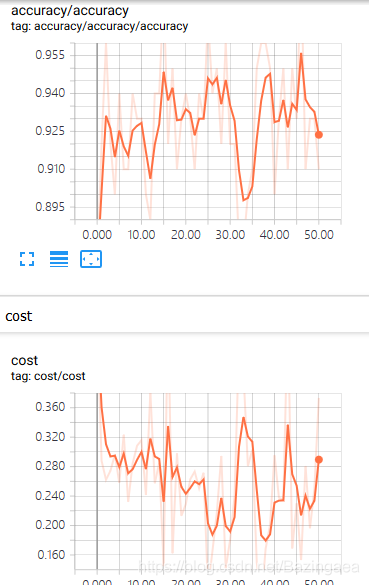
SCALARS中放了很多这样的表，准确度，代价函数，以及参数值，都是随着迭代次数的变化而变化

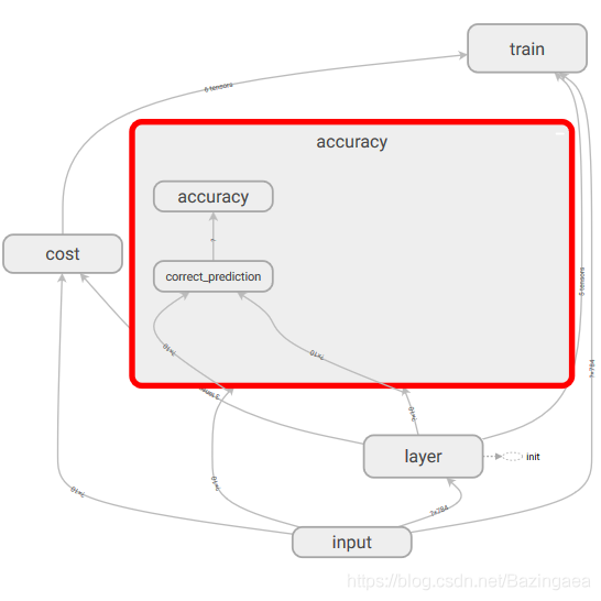
GRAPHS中放着网络的图结构，可以将某个子模块点开看细节，也可以将子模块脱离整体，或者将脱离整体的模块整合在一起，通过单击右键就可以看到操作提示。

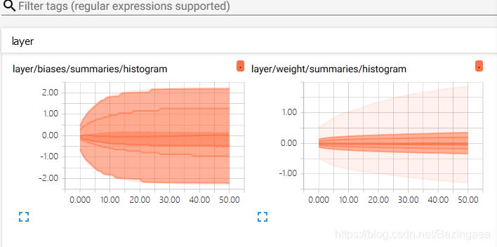
DISTRIBUTION中放了参数w和b的分布图：

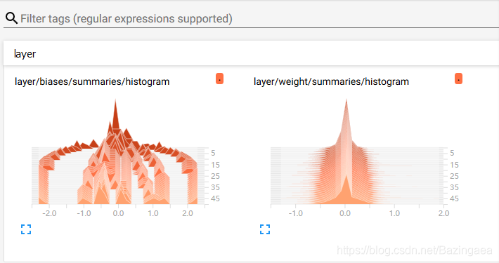
HISTOGRAM中放了参数的直方图：